INTRODUCTION
Background
Currently, our daily life is profoundly impacted by the outbreak of the Coronavirus disease 2019 (COVID-19), and the number of confirmed cases has quickly increased in the past few weeks. Starting mid-March, states, companies, businesses, and schools are beginning to take action to respond to the outbreak. States are promoting residents to stay at home, companies are promoting remote working, businesses are starting to suspend their operations, and schools are beginning to transition to e-learning. All of these are acting as a part of social distancing. Research shows that social distancing can highly reduce the infection rate of infectious diseases. A model shows that if 25% of the residents reduce daily social interactions by 50%, the number of primary infections can be reduced by 81% (Maharaj).
Orienting Material
a. Using a Quadratic Least Squares polynomial to discover the formula modeling the new cases of COVID-19 over a period of time.
b. Using Richardson’s Extrapolation to the 3-point midpoint formula to calculate the increased rate of new cases of COVID-19.
c. Generating a report for the time period every 7 days starting January 21st.
Thesis
Even though some people believe the Coronavirus is less serious or that quarantine at home has no effect, the purpose of this report is to raise more people’s attention to the new Coronavirus and encourage people to isolate at home. Compared with before, people began to pay attention to the severity of the Coronavirus, and many people began to isolate themselves, resulting in a significant drop in the rate of new patients.
ANALYSIS
Data Collection
a. Our data are collected from the 2019 Novel Coronavirus COVID-19 (2019-nCoV) Data Repository by Johns Hopkins CSSE, which aggregated data from the WHO, CDC, ECDC, NHC, DXY, 1point3acres, Worldometers.info, BNO, the COVID Tracking Project, state and national government health departments, and local media reports (Dong). They also promise that the data will be updated frequently. The data provided contains the Federal Information Processing Standards (FIPS) code (Dong); County name; Province, state, or dependency name; Update time; Geocode; Confirmed case number; Deaths case number; Recovered number; and Active number. In summary, the source is credible and usable.
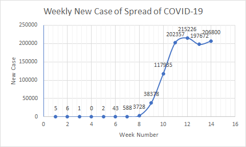
b. Data Table
| Week Number | Start Date | End Date | New Cases | Total Cases |
| Week1 | 01-21-20 | 01-27-20 | 5 | 5 |
| Week2 | 01-28-20 | 02-03-20 | 6 | 11 |
| Week3 | 02-04-20 | 02-10-20 | 1 | 12 |
| Week4 | 02-11-20 | 02-17-20 | 0 | 12 |
| Week5 | 02-18-20 | 02-24-20 | 2 | 14 |
| Week6 | 02-25-20 | 03-02-20 | 43 | 57 |
| Week7 | 03-03-20 | 03-09-20 | 588 | 645 |
| Week8 | 03-10-20 | 03-16-20 | 3728 | 4373 |
| Week9 | 03-17-20 | 03-23-20 | 38378 | 42751 |
| Week10 | 03-24-20 | 03-30-20 | 117935 | 160686 |
| Week11 | 03-31-20 | 04-06-20 | 202357 | 362952 |
| Week12 | 04-07-20 | 04-13-20 | 215226 | 578178 |
| Week13 | 04-14-20 | 04-20-20 | 197672 | 775850 |
| Week14 | 04-21-20 | 04-27-20 | 206800 | 982650 |
c. Data Graph
Quadratic Least Squares Polynomial
1 | %% Quadratic least squares polynomial |
^Download MATLAB Code for Quadratic least squares polynomial
^Download MATLAB Code for Cubic least squares polynomial
Model: $$f(x)=(-25.91048)(x)^2+(4572.54925)x-171258.00999$$
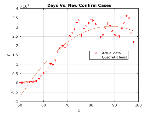
Although the data we have is somewhat noisy, we can still generate a reasonable model formula by using the Quadratic Least Squares polynomial. We can use the generated polynomial and apply it to Richardson’s Extrapolation using the 3-point midpoint formula.
Richardson’s Extrapolation to the 3-point Midpoint
Once we get a formula using the Quadratic Least Squares polynomial, we can use Richardson’s Extrapolation to the 3-point midpoint formula to find its first derivative. In numerical analysis, the Richardson extrapolation method can improve the convergence efficiency of a series or sequence. Furthermore, Richardson’s extrapolation method can generate high-precision results even when using low-order formulas (Burden, 185).
The formula we have is $f(x)=(-25.91048)(x)^2+(4572.54925)x-171258.00999$.
1 | import java.util.Scanner; |
^Download Python Code for Richardson 3-point midpoint formula
Input day = 60, with h = 4:
result: 1463.2916425999992
result: 1463.2916499999992
result: 1463.2916500000138
$N_1 (4)=1463.2916425999992$
$N_1 (2)=1463.2916499999992$
$N_1 (1)=1463.2916500000138$
$N_2 (2)=N_1 (1)+\frac{1}{3} [N_1 (1)-N_1 (2)]=1463.29165+\frac{1}{3} [1463.29165-1463.29165]=1463.29165$
$N_2 (4)=N_1 (2)+\frac{1}{3} [N_1 (2)-N_1 (4)]=1463.29165+\frac{1}{3} [1463.29165-1463.29164]=1463.29165$
$N_3 (4)=N_2 (2)+\frac{1}{5} [N_2 (2)-N_2 (4)]=1463.29165+\frac{1}{5} [1463.29165-1463.29165]=1463.29165$
Input day = 70, with h = 4:
$N_1 (4)=945.0820499999973$
$N_1 (2)=945.0820499999973$
$N_1 (1)=945.0820499999973$
$N_2 (2)=N_1 (1)+\frac{1}{3} [N_1 (1)-N_1 (2)]=945.08205+\frac{1}{3} [945.08205-945.08205]=945.08205$
$N_2 (4)=N_1 (2)+\frac{1}{3} [N_1 (2)-N_1 (4)]=945.08205+\frac{1}{3} [945.08205-945.08205]=945.08205$
$N_3 (4)=N_2 (2)+\frac{1}{5} [N_2 (2)-N_2 (4)]=945.08205+\frac{1}{5} [945.08205-945.08205]=945.08205$
Input day = 80, with h = 4:
$N_1 (4)=426.8724499999953$
$N_1 (2)=426.87245000000985$
$N_1 (1)=426.87244999998074$
$N_2 (2)=N_1 (1)+\frac{1}{3} [N_1 (1)-N_1 (2)]=426.87245+\frac{1}{3} [426.87245-426.87245]=426.87245$
$N_2 (4)=N_1 (2)+\frac{1}{3} [N_1 (2)-N_1 (4)]=426.87245+\frac{1}{3} [426.87245-426.87245]=426.87245$
$N_3 (4)=N_2 (2)+\frac{1}{5} [N_2 (2)-N_2 (4)]=426.87245+\frac{1}{5} [426.87245-426.87245]=426.87245$
Input day = 90, with h = 4:
$N_1 (4)=-91.33715000000302$
$N_1 (2)=-91.33715000000666$
$N_1 (1)=-91.33715000000666$
$N_2 (2)=N_1 (1)+\frac{1}{3} [N_1 (1)-N_1 (2)]=-91.33715+\frac{1}{3} [-91.33715+91.33715]=-91.33715$
$N_2 (4)=N_1 (2)+\frac{1}{3} [N_1 (2)-N_1 (4)]=-91.33715+\frac{1}{3} [-91.33715+91.33715]=-91.33715$
$N_3 (4)=N_2 (2)+\frac{1}{5} [N_2 (2)-N_2 (4)]=-91.33715+\frac{1}{5} [-91.33715+91.33715]=-91.33715$
CONCLUSION
Summary
Two methods are applied in this project: the Quadratic Least Squares polynomial and Richardson’s Extrapolation to the 3-point midpoint formula. The Quadratic Least Squares polynomial is used to discover the underlying formula, and Richardson’s Extrapolation to the 3-point midpoint formula is used to discover the case increase rate. A graph is generated when the Quadratic Least Squares polynomial is calculated in MATLAB, which clearly shows the polynomial approximation of the COVID-19 outbreak over time.
Accuracy
By analyzing the data, we can easily find that the data is extremely noisy, which limits the usage of certain methods in Numerical Analysis. However, polynomial least squares regression can solve this problem; it can generate a low-degree polynomial that can be used to estimate an underlying polynomial trend (Kalman).
When we use Richardson’s extrapolation method for our data analysis, we can see that the results are increasingly converging to the real derivative solution of the generated formula.
Conclusion
From our analysis results above, the Quadratic Least Squares polynomial can provide us with the best-fit line even though we have noisy data. Since many organizations and schools encourage people to isolate themselves, the results from the 60th, 70th, 80th, and 90th days—which give us the derivative of the formula (representing the rate of increase)—show that the rate of new cases is continuously decreasing. We can easily conclude that with the effort of social distancing, including the hard work of government officials, medical workers, and all residents in the US, the infection rate will drop into a stable stage and will gradually disappear.
Reference
- Burden, Richard L., and J. Douglas. Faires. Numerical Analysis. Brooks/Cole, Cengage Learning, 2011.
- Dong, Ensheng, et al. “An Interactive Web-Based Dashboard to Track COVID-19 in Real Time.” The Lancet Infectious Diseases, 19 Feb. 2020, www.thelancet.com/journals/laninf/article/PIIS1473-3099(20)30120-1.
- Kalman, R. E. “A New Approach to Linear Filtering and Prediction Problems.” Journal of Basic Engineering, American Society of Mechanical Engineers Digital Collection, 1 Mar. 1960, https://asmedigitalcollection.asme.org/fluidsengineering/article-abstract/82/1/35/397706/A-New-Approach-to-Linear-Filtering-and-Prediction.
- Maharaj, Savi, and Adam Kleczkowski. “Controlling Epidemic Spread by Social Distancing: Do It Well or Not at All.” BMC Public Health, 20 Aug. 2012, https://bmcpublichealth.biomedcentral.com/articles/10.1186/1471-2458-12-679.